Gumbel-Max Trick Inference
There has been recently two concurrent works on using a relaxed version of the Gumbel-Max Trick to train deep probabilistic models (The Concrete Distribution: A Continuous Relaxation of Discrete Random Variables and Categorical Reparameterization with Gumbel-Softmax). I like to compare the Gumbel-Max trick, as described in this blogpost, to the Reparametrization Trick (previously referred to as Backpropagating through Random Number Generators) as it decomposes sampling from a parametrized distribution into two parts: sampling from a standard distribution and a deterministic parametrized function, possibly resulting in accelerated sampling.
The Gumbel-Max Trick is a method to sample from a categorical distribution \(\text{Cat}(\alpha_1, \alpha_2, \dots, \alpha_K)\), where category \(k\) has \(\alpha_k\) probability to be sampled among K categories, and relies on the Gumbel distribution defined by the Cumulative Distribution Function:
\[CDF_{Gumbel}(\epsilon) = \exp\big(-\exp(-\epsilon)\big)\]This trick is based on the clever observation that, if \((\epsilon_1, \epsilon_2, \dots, \epsilon_K)\), then \(k_{max} = \text{argmax}_{k' \leq K}\big(\epsilon_{k'} + \log(\alpha_{k'})\big)\) follows the desired categorical distribution \(\text{Cat}(\alpha_1, \alpha_2, \dots, \alpha_K)\) (see this blogpost from Ryan Adams for proof). In practice, we can sample from this Gumbel distrbution using auxiliary random uniform variables \(u\) in \([0, 1]\) using inverse transform sampling:
\[u \sim \mathcal{U}\big([0, 1]\big) \\ \epsilon = CDF_{Gumbel}^{-1}(u) = -\log\big(-\log(u)\big)\]Last summer, Luke Vilnis asked me whether it was possible to practically infer those Gumbel random variables \((\epsilon_1, \epsilon_2, \dots, \epsilon_K)\) given an observed category \(k\). That is: what is the expression of the posterior distribution \(p\big(\epsilon_1, \dots, \epsilon_k, \dots, \epsilon_K \mid K_{max} = k\big)\) and how to sample from it ? As a thought experiment, I will describe in this blogpost how to do it.
Uniform reparametrization
If we choose to be interested in the associated uniform random variables \(u_{k'} = CDF_{Gumbel}(\epsilon_{k'})\), inference of those latent variables looks conceptually easier. Indeed, given the observed category \(k\), \(p(u_1, u_2, \dots, u_K \mid K_{max} = k)\) can be more easily derived through Bayes Rule. If we consider the set
\[\mathcal{C}_k = \big\{(u_1, u_2, \dots, u_K), \forall k' \leq K, ~~ \epsilon_{k'} + \log(\alpha_{k'}) \leq \epsilon_{k} + \log(\alpha_{k})\big\} \\ = \big\{(u_1, u_2, \dots, u_K), \forall k' \leq K, \\ ~~ -\log\big(-\log(u_{k'})\big) + \log(\alpha_{k'}) \leq -\log\big(-\log(u_{k})\big) + \log(\alpha_{k})\big\},\]then:
- \(p(K_{max} = k \mid u_1, u_2, \dots, u_K) = \mathbb{1}_{\mathcal{C}_k}\big((u_1, u_2, \dots, u_K)\big)\);
- \(p(u_1, u_2, \dots, u_K) = 1\) because \(u_{k'}\) follow a priori the uniform distribution \(\mathcal{U}\big([0, 1]^{K}\big)\);
- \(p(K_{max} = k) = \alpha_k\) by definition of \(\text{Cat}(\alpha_1, \alpha_2, \dots, \alpha_K)\).
Therefore, we have
\(p(u_1, u_2, \dots, u_K \mid K_{max} = k) = \frac{p(K_{max} = k \mid u_1, u_2, \dots, u_K)p(u_1, u_2, \dots, u_K)}{p(K_{max} = k)} \\ = \alpha_{k}^{-1} \mathbb{1}_{\mathcal{C}_k}\big((u_1, u_2, \dots, u_K)\big)\) Meaning that \(p(u_1, u_2, \dots, u_K \mid K_{max} = k)\) is uniform in the set defined by the nonlinear constraints
\[\forall k' \leq K, ~~ -\log\big(-\log(u_{k'})\big) + \log(\alpha_{k'}) \leq -\log\big(-\log(u_{k})\big) + \log(\alpha_{k})\]of volume \(\alpha_k\).
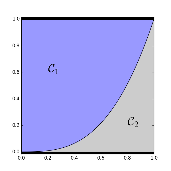
 2-D example of how \(\mathcal{C}_1\) and \(\mathcal{C}_2\) partition the space of \((u_1, u_2)\) configurations with \(\alpha_1 = .75\) and \(\alpha_2 = .25\).
Sampling
Usually, when we sample from a uniform distribution, it is usually from an axis-aligned box from which it’s very easy to sample like \([0, 1]^{K}\). But in general, sampling from an arbitrary uniform distribution can be non-trivial and requires more complex sampling procedure like Markov Chain Monte Carlo algorithms, especially since \(\mathcal{C}_1, \dots, \mathcal{C}_K\) define a partition with nonlinear boundaries. In this case, you will see a derivation of an exact Monte Carlo procedure from the described constraints.
\[\forall k' \leq K, ~~ -\log\big(-\log(u_{k'})\big) + \log(\alpha_{k'}) \leq -\log\big(-\log(u_{k})\big) + \log(\alpha_{k}) \\ \Leftrightarrow -\log\big(-\log(u_{k'})\big) \leq -\log\big(-\log(u_{k})\big) + \log\left(\frac{\alpha_{k}}{\alpha_{k'}}\right) \\ \Leftrightarrow u_{k'} \leq \exp\Big(-\exp\Big(\log\big(-\log(u_{k})\big) + \log\left(\frac{\alpha_{k'}}{\alpha_{k}}\right)\Big)\Big) \\ \Leftrightarrow u_{k'} \leq \exp\Big(\frac{\alpha_{k'}}{\alpha_{k}}\log(u_{k})\Big) \\ \Leftrightarrow 0 \leq u_{k'} \leq u_{k}^{\frac{\alpha_{k'}}{\alpha_{k}}} \leq 1\]Meaning that \(\forall k' \neq k, ~~ p\big(u_{k'} \mid K_{max} = k, u_{k}\big) = \mathcal{U}\big([0, u_{k}^{\frac{\alpha_{k'}}{\alpha_{k}}}]\big)\). Finally, we derive the expression of \(p(u_{k} \mid K_{max} = k)\) in \(\mathcal{C}_k\):
\[p\big(u_1, \dots, u_k, \dots, u_K \mid K_{max} = k\big) = \alpha_{k}^{-1} \\ \Leftrightarrow p\big(u_1, \dots, u_{k-1}, u_{k+1}, \dots, u_K \mid K_{max} = k, u_{k}\big) p(u_{k} \mid K_{max} = k) = \alpha_{k}^{-1} \\ \Leftrightarrow \prod_{k' \neq k}p\big(u_{k'} \mid K_{max} = k, u_{k}\big) p(u_{k} \mid K_{max} = k) = \alpha_{k}^{-1} \\ \Leftrightarrow \prod_{k' \neq k}\mathcal{U}\big([0, u_{k}^{\frac{\alpha_{k'}}{\alpha_{k}}}]\big) p(u_{k} \mid K_{max} = k) = \alpha_{k}^{-1} \\ \Leftrightarrow \prod_{k' \neq k}{u_{k}^{-\frac{\alpha_{k'}}{\alpha_{k}}}} p(u_{k} \mid K_{max} = k) = \alpha_{k}^{-1} \\ \Leftrightarrow u_{k}^{-\sum_{k' \neq k}{\frac{\alpha_{k'}}{\alpha_{k}}}} p(u_{k} \mid K_{max} = k) = \alpha_{k}^{-1} \\ \Leftrightarrow u_{k}^{\frac{\alpha_{k} - 1}{\alpha_{k}}} p(u_{k} \mid K_{max} = k) = \alpha_{k}^{-1} \\ \Leftrightarrow p(u_{k} \mid K_{max} = k) = \alpha_{k}^{-1} u_{k}^{\frac{1 - \alpha_{k}}{\alpha_{k}}} \\ \Leftrightarrow p(u_{k} \mid K_{max} = k) = \alpha_{k}^{-1} u_{k}^{\alpha_{k}^{-1} - 1} \\ \Leftrightarrow CDF(u_{k} \mid K_{max} = k) = u_{k}^{\alpha_{k}^{-1}}\]Once again, we can efficiently sample from this posterior distribution using auxiliary random uniform variables \(v_{k'}\) through inverse transform sampling:
\[\forall k' \leq K, ~~ v_{k'} \sim \mathcal{U}\big([0, 1]\big) \\ u_{k} = v_{k}^{\alpha_{k}} \\ \forall k' \neq k, ~~ u_{k'} = u_{k}^{\frac{\alpha_{k'}}{\alpha_{k}}} v_{k'} = v_{k}^{\alpha_{k'}} v_{k'}\]If you were to infer the Gumbel variables \((\epsilon_1, \epsilon_2, \dots, \epsilon_K)\), then \(\epsilon_{k'} = -\log\big(-\log(u_{k'})\big)\).
Acknowledgements
I’m very grateful to Luke Vilnis, Vincent Dumoulin, Kyle Kastner, Harm de Vries and my supervisors, Yoshua Bengio and Samy Bengio, for interesting discussions that were helpful in writing this post. I discovered the Gumbel-Max Trick through the NIPS 2014 paper A* sampling.